Harmonizing Climate and Population Data with Inverse Distance Weighting Interpolation Method

By Pavel Pashagin

Recently we added the Kontur Nighttime Heatwave Risk layer to Disaster Ninja. It shows heat-stress risk areas with night-time temperatures above 25°C. It was created using Kontur Population dataset and Probable Futures climate model. The combination of these datasets can give us a lot of useful information, but we had to make them compatible first.

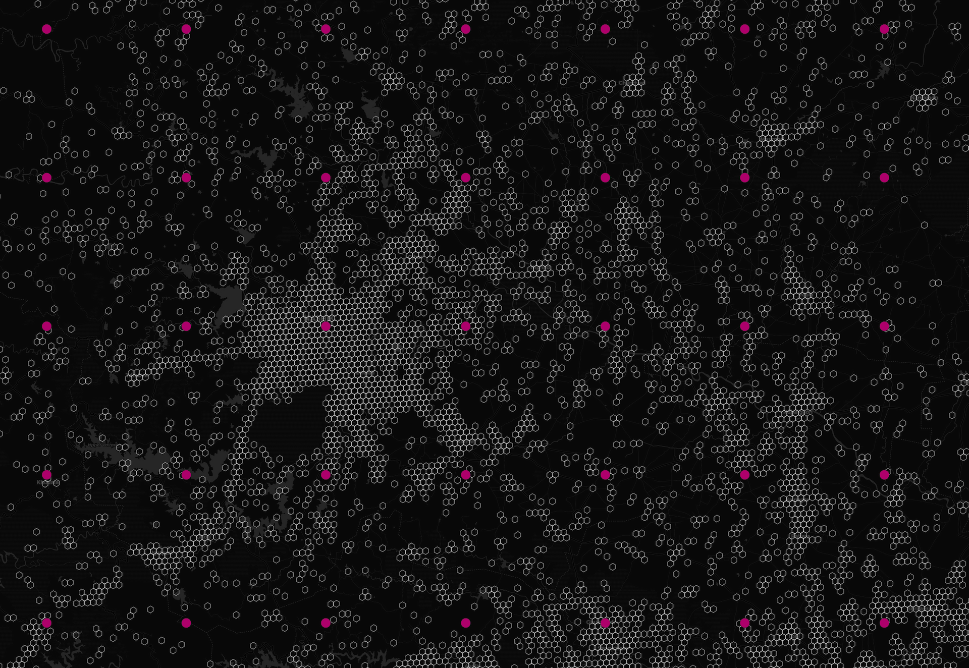
The main problem that arose when working with them was the different scales of the source data. Kontur Population dataset is built using H3 hexagons at resolution 8 with the average hexagon area of 0.7373 km² and the average hexagon edge length of 0.4613 km.

The data from Probable Futures model is represented in 22-kilometer squares called grid-cells. It is sourced from the CORDEX-CORE framework, a standardization for regional climate model output.

H3 gridded Kontur Population data and point layer with climate data

To make both datasets compatible we need to bring the Probable Futures data to the H3 hexagonal grid of the resolution we use for population density data. To do so we use the Inverse Distance Weighting (IDW) interpolation method, PostgreSQL bindings for H3, and some SQL.

First, let’s make a grid with hexagons for areas, where we have data, i.e. at least one point from the Probable Futures dataset so we don’t need to make calculations for unpopulated areas in the ocean or for areas with no data. The closest H3 resolution is level 4 (average hexagon edge length is 22.6063 km):

create table pf_grid_h3_r4 as (select distinct h3_geo_to_h3(geom, 4) as h3 from pf_data);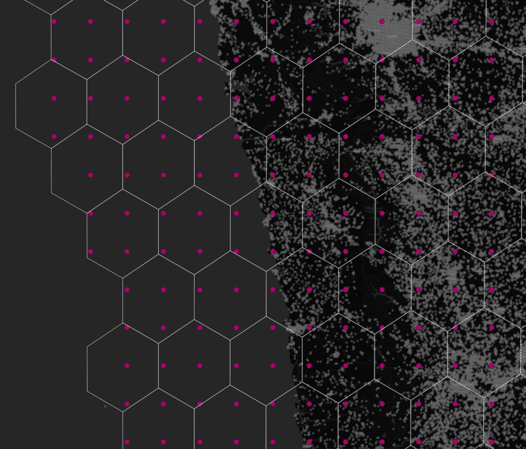

Next, we have 2 ways to proceed:

The longer one is to divide the resulting hexagons into smaller 8th-level ones right away and interpolate on it.
The faster one is to perform interpolation at the level below (5th one) and transfer these results to all child levels up to the 8th.

In fact, none of these ways is perfect. The interpolation at the 5th level is too rough, and it takes an unacceptably long time for our ETL process to perform it at the 8th level. The compromise is to make interpolation at the 7th level.

create table pf_grid_h3_r7 as (
   select distinct 
      h3_to_children(h3, 7)           as h3,   
      h3_to_children(h3, 7)::geometry as geom
   from pf_grid_h3_r4
);
create index on pf_grid_h3_r7 using gist (geom);

The query for calculations at level 8 would look similar, but it would take significantly longer than the statement_timeout settings set in our PostgreSQL database.

create table pf_grid_h3_r8 as (
    select distinct
        h3_to_children(h3, 8)           as h3,
        h3_to_children(h3, 8)::geometry as geom
    from pf_grid_h3_r4
);

Now we can calculate the values in each hexagon using the IDW method:

create table pf_data_idw_r7 as (
with nearest_points as (
    select h3,
           dist,
           days_mintemp_above_25c_1c
    from pf_grid_h3_r7 
         cross join lateral (
            select 
               days_mintemp_above_25c_1c,
               ST_Distance(pf_grid_h3_r7.geom::geography, pf_data.geom::geography) AS dist
            from pf_data
            order by pf_data.geom <-> pf_grid_h3_r7.geom
            limit 4
        ) grid
)
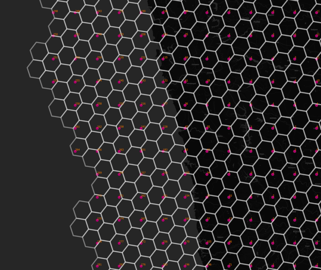
select h3,
       7::integer as resolution,
       floor((sum(days_mintemp_above_25c_1c / dist) / sum(1 / dist))) as days_mintemp_above_25c_1c
from nearest_points
group by h3);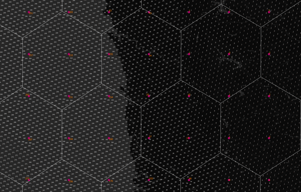

And finally, we can fill up the hexagons at resolution 8 with obtained numbers:

create table pf_data_h3_r8 as (
    select 
        h3_to_children(h3, 8) as h3,
        days_mintemp_above_25c_1c,
        8::integer as resolution
    from pf_data_idw_r7
);

These numbers can now be used for calculations with Kontur Population and other hexagonal datasets at resolution 8.